Lecture 26: Fast Fourier Transform (FFT)

Analyzing Data

Given some data, we often need to ask:

What is the nature of the data?
What is the period?
Can we rid the data of noise?

Real-World Examples

Signal Processing

Remove (high-frequency) noise in an input signal.

Weather Data

Data often contains different cycles:

Daily data
Yearly data
Goal: Isolate one of these.

Economics

Seasonal adjustment: remove unwanted periodicities to reveal "secular" trends.

Audio

Digital filtering in audio.

Convolution & Correlation

Discrete convolution of two sequences of data $u$ and $v$ of length $n$:

$$ \{u \star v\}_m = \sum_{k=0}^{n-1} v_k u_{m-k},\quad m = 0,1,\dots,n-1 $$

This relates to cross correlation of two sequences or autocorrelation with self.

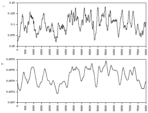
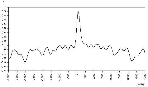
Image Registration

Aligning a sub-image with another image.

Other Applications

Spectral Analysis
Data compression
Partial Differential Equations
Multiplication of polynomials

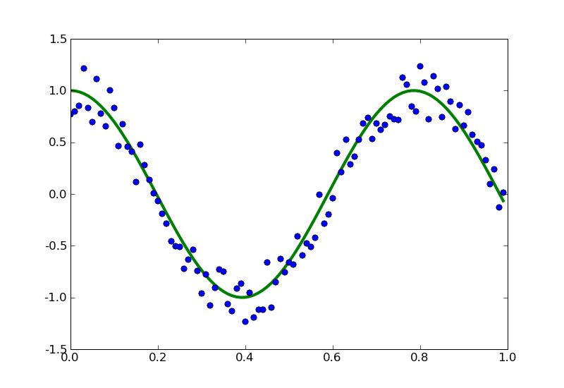
Interpolation by Trigonometry

When we have periodic data, use periodic interpolating functions: sines, cosines, etc.
Decompose a function into a combination of sines and cosines (as we did with polynomial basis functions).
Decomposing into (co)sines of different "frequencies" naturally orders the data.
The gist: working in a frequency (transformed) space is easier (faster) than the time domain.

Recall Fourier Series

Suppose $f(x)$ is periodic on $[-\pi,\pi]$. The Fourier Series for $f(x)$ is:

$$ f(x) \approx \frac{a_0}{2} + \sum_{n=1}^{\infty} a_n \cos(nx) + b_n \sin(nx) $$

with coefficients:

$$ a_n = \frac{1}{\pi} \int_{-\pi}^{\pi} f(x) \cos(nx)\, dx \quad b_n = \frac{1}{\pi} \int_{-\pi}^{\pi} f(x) \sin(nx)\, dx $$

Example: Sawtooth Wave

$f(x) = x$ on $[-\pi,\pi]$.

Then $a_n = 0$ (odd function) and $b_n = 2 \frac{(-1)^{n+1}}{n}$.

$$ f(x) = 2\sum_{n=1}^{\infty} \frac{(-1)^{n+1}}{n} \sin(nx) $$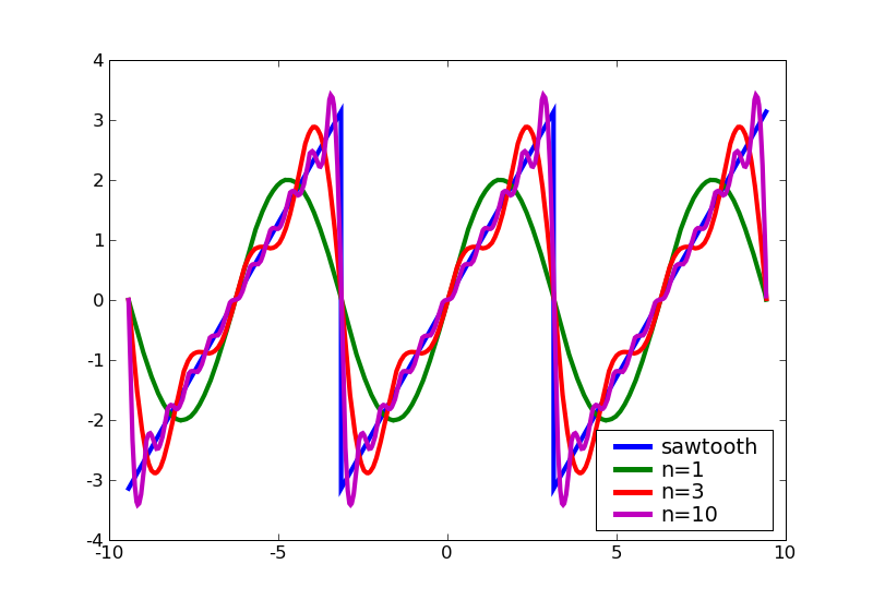

General Fourier Notation

Use complex exponential notation using Euler's Identity:

$$ e^{i x} = \cos(x) + i \sin(x),\qquad i = \sqrt{-1} $$

Pure cosine and sine can be written as:

$$ \cos(x) = \frac{e^{i x} + e^{-ix}}{2},\quad \sin(x) = \frac{e^{i x} - e^{-ix}}{2i} $$

Then a Fourier Series on interval $[a,b]$ with period $\tau$ is:

$$ g(x) = \sum_{n=-\infty}^{\infty} G_n e^{i 2 \pi n x / \tau} $$

with:

$$ G_n = \frac{1}{\tau} \int_{a}^{b} g(x) e^{-i 2\pi n x / \tau}\, dx $$

Roots of Unity

A primitive $n^{th}$ root of unity for integer $n$ is given by:

$$ \omega_n = \cos\left(\frac{2\pi}{n}\right) - i \sin\left(\frac{2\pi}{n}\right) = e^{-\frac{2\pi i}{n}} $$

The $n^{th}$ roots of unity are called twiddle factors here and are given by $\omega_n^k$ or $\omega_n^{-k}$, $k=0,\dots,n-1$.

The Discrete Fourier Transform

The DFT of sequence $x = [x_0,\dots,x_{n-1}]^T$ is a sequence $y = [y_0,\dots,y_{n-1}]^T$ given by:

$$ y_m = \sum_{k=0}^{n-1} x_k \omega_n^{mk}, \quad m=0,1,\dots,n-1 $$

In matrix notation this is:

$$ y = F_n x,\qquad \{F_n\}_{mk} = \omega_n^{mk} $$

Example with $n=4$:

$$ F_4 = \begin{bmatrix} 1 & 1 & 1 & 1\\ 1 & \omega^1 & \omega^2 & \omega^3\\ 1 & \omega^2 & \omega^4 & \omega^6\\ 1 & \omega^3 & \omega^6 & \omega^9\\ \end{bmatrix} = \begin{bmatrix} 1 & 1 & 1 & 1\\ 1 & -i & -1 & i\\ 1 & -1 & 1 & -1\\ 1 & i & -1 & -i\\ \end{bmatrix} $$

Inverse DFT

Note that $F_4 \cdot F_4^*$ (conjugate transpose) yields a scaled identity. Specifically:

$$ F_n^{-1} = \frac{1}{n} F_n^{*} $$

Thus the Inverse DFT is:

$$ x_k = \frac{1}{n} \sum_{m=0}^{n-1} y_m \omega_n^{-mk}, \quad k=0,1,\dots,n-1 $$

Result: DFT and IDFT give trigonometric interpolation using only a mat-vec operation $\mO(n^2)$.

DFT Properties

The DFT $y$ of a real sequence $x$ is generally complex.
Components of $y$ are conjugate symmetric: $y_k = \bar{y}_{n-k}$ for $k=1,\dots, (n/2)-1$.
Special Components:
- $y_0$: Sum of components (Zero frequency / DC component).
- $y_{n/2}$: Highest representable frequency (Nyquist frequency).

DFT Examples

Random Sequence

For $x = [4, 0, 3, 6, 2, 9, 6, 5]^T$, $y = F_8 x$:

y = [35.0, -5.1+8.7i, -3.0+2.0i, 9.1+2.7i, -5.0, 9.1-2.7i, -3.0-2.0i, -5.1-8.7i]^T

Note: $y_0$ is real (sum), $y_4$ is real. $y_5, y_6, y_7$ are conjugates of $y_3, y_2, y_1$.

Cyclic Sequence

For $x = [1, -1, 1, -1, 1, -1, 1, -1]^T$:

y = [0, 0, 0, 0, 8, 0, 0, 0]^T

Sequence $x$ has the highest oscillation rate. $y$ has only a nonzero component at the Nyquist frequency ($y_4$).

Goal: Efficiency

We want to take advantage of symmetries. Consider $n=4$:

$$ y_m = \sum_{k=0}^3 x_k \omega_n^{mk} $$

Using properties like $\omega_n^0 = 1, \omega_n^2 = -1$, we can simplify:

\begin{align*} y_0 & = (x_0 + x_2) + \omega_n^0 (x_1 + x_3)\\ y_1 & = (x_0 - x_2) + \omega_n^1 (x_1 - x_3)\\ y_2 & = (x_0 + x_2) + \omega_n^2 (x_1 + x_3)\\ y_3 & = (x_0 - x_2) + \omega_n^3 (x_1 - x_3)\\ \end{align*}

This reduces operations from 12 adds/16 mults to 8 adds/6 mults.

Recursive Structure

Computing the 4-point DFT reduced to computing the DFT of its two 2-point even and odd subsequences.

Key Insight:

The DFT of an $n$-point sequence can be computed by two $n/2$-point DFTs ($n$ even).

Let $P_n$ be a permutation matrix that groups even then odd columns. Then:

$$ F_4 P_4 = \begin{bmatrix} F_2 & D_2 F_2 \\ F_2 & -D_2 F_2 \end{bmatrix} $$

where $D_2 = \text{diag}(1, \omega_4 = -i)$.

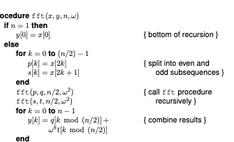
The FFT Algorithm

This holds for any even $n$. In general:

$P_n$ groups even then odd numbered columns.
$D_{n/2} = \text{diag}(1, \omega_n, \dots, \omega_n^{(n/2)-1})$.
To apply $F_n$, apply $F_{n/2}$ to even/odd subsequences.
Scale results by $\pm D_{n/2}$.

This recursive DFT is called the Fast Fourier Transform (FFT).

Complexity & Features

Cost: $\log_2 n$ levels of recursion, with $\mO(n)$ operations each. Total: $\mO(n \log n)$.
Often computed in-place.
More reductions if $x$ is real.
Can be written iteratively.