Linear Solvers

Iterative Methods

Solving $Ax=b$ by successive approximation: Jacobi, Gauss-Seidel, and Conjugate Gradients.

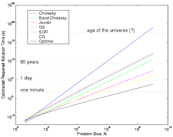
Direct Solvers: Complexity Recap

Before diving into iterative methods, let's review the cost of direct methods for $Ax=b$.

System Type	Complexity
Diagonal	$\mathcal{O}(n)$
Tridiagonal	$\mathcal{O}(n)$
Triangular (Forward/Back Sub)	$\mathcal{O}(n^2)$
Banded ($m$-band)	$\mathcal{O}(m^2 n)$
Full System (GE / LU)	$\mathcal{O}(n^3)$

Approximate Solutions

What if we don't need the exact solution $x^*$? We seek an approximation $\hat{x}$ such that $\|\hat{x} - x^*\| \le \epsilon$.

The Residual

We can't calculate the error $e = x^* - \hat{x}$ directly (since we don't know $x^*$). Instead, we use the residual:

$\hat{r} = b - A\hat{x}$

Note: $\hat{r} = A e$.

Measuring Size

How "big" is the residual? Use norms:

$\|r\|_1 = \sum |r_i|$
$\|r\|_2 = \sqrt{\sum r_i^2}$
$\|r\|_\infty = \max |r_i|$

Iterative Strategy

Given a guess $x^{(0)}$, how do we improve it?

Ideally: $x^{(1)} = x^{(0)} + A^{-1}r^{(0)}$. But computing $A^{-1}$ is too expensive.

Strategy: Approximate $A^{-1}$ with a matrix $Q^{-1}$ that is cheap to compute.

$x^{(k)} = x^{(k-1)} + Q^{-1}r^{(k-1)}$

Jacobi Method

Approximates $A$ with its diagonal $D$.

Q = diag(A)
for k = 1:max_iter
    r = b - A*x
    if norm(r) < tol, break x=x + r ./ diag(A) end

Gauss-Seidel Method

Approximates $A$ with its lower triangle ($D-L$). Uses updated values immediately.

Q = tril(A) % Lower triangular
for k = 1:max_iter
    r = b - A*x
    if norm(r) < tol, break % Solve Q*delta=r efficiently x=x + forward_sub(Q, r) end

Convergence

When do these methods work? Let's look at the error propagation.

$e^{(k)} = (I - Q^{-1}A) e^{(k-1)}$

Condition for Convergence

The iteration converges if the spectral radius of the iteration matrix is less than 1:

$\| I - Q^{-1}A \| < 1$

Sufficient Condition

If $A$ is Diagonally Dominant ($|a_{ii}| > \sum_{j \ne i} |a_{ij}|$), then Jacobi and Gauss-Seidel guaranteed to converge.

Conjugate Gradients (CG)

For Symmetric Positive Definite (SPD) matrices, we can view solving $Ax=b$ as minimizing the quadratic function: \[ \phi(x) = \frac{1}{2} x^T A x - x^T b \]

The Idea

Instead of going down the steepest gradient (which zig-zags), we search in conjugate directions. This guarantees convergence in at most $n$ steps (in exact arithmetic).

% Conjugate Gradient Algorithm
x = x0
r = b - A*x
s = r
for k = 1:n
    alpha = (r'*r) / (s'*A*s)
    x = x + alpha * s
    r_new = r - alpha * A * s
    beta = (r_new'*r_new) / (r'*r)
    s = r_new + beta * s
    r = r_new
end

🧠 Final Challenge +20 XP

Which method updates the solution vector using the most recent values available within the same iteration step?