Lecture 5: Matrix, Vector Operations

🎯 Goals

1 Recall linear algebra (ouch!).
2 Cost analysis of basic operations.
3 Identify basic solution schemes to systems.

Why this matters

Matrix problems arise in graphics, design, information sciences.
BLAS (Basic Linear Algebra Subprograms) is the standard.
Simple systems set the stage for avoiding errors and large costs.

⚠️

Prerequisite Warning

Linear Algebra is a prerequisite! You should be comfortable with Appendix D.1 and D.2 in the textbook.

1

The Matrix Inverse

Let $A$ be a square (\matdim{n}{n}) matrix. The inverse $A^{-1}$ satisfies:

$A^{-1}A = I \quad \text{and} \quad AA^{-1} = I$

Formal Solution to $Ax=b$

\begin{align*} Ax &= b \\ A^{-1} A x &= A^{-1}b \\ Ix &= A^{-1}b \\ x &= A^{-1}b \end{align*}

🚫 STOP!

Do not compute the solution to $Ax=b$ by finding $A^{-1}$ and multiplying!

We see: $x = A^{-1}b$.
We do: Solve $Ax=b$ by Gaussian elimination.

🧠 Knowledge Check +10 XP

Why do we avoid computing the matrix inverse explicitly to solve a system?

2

Singularity & Solution Existence

Singular Matrix Properties

If $A$ is singular:

Columns/Rows are linearly dependent.
$\rank{A} < n$.
$\det(A) = 0$.
$A^{-1}$ does not exist.
Solution may not exist or is not unique.

Requirement for Unique Solution

The solution to $Ax=b$ exists and is unique for any $b$ if and only if:

$\rank{A} = n$

Three Situations for $Ax=b$

1. Unique Solution

$A$ is Nonsingular.

$A=\begin{bmatrix}2&0\\0&4\end{bmatrix}, b=\begin{bmatrix}1\\8\end{bmatrix}$
$\Rightarrow x=\begin{bmatrix}1/2\\2\end{bmatrix}$

2. Infinite Solutions

$A$ singular, $b \in Range(A)$.

$A=\begin{bmatrix}2&0\\0&0\end{bmatrix}, b=\begin{bmatrix}1\\0\end{bmatrix}$
$\Rightarrow x=\begin{bmatrix}1/2\\\alpha\end{bmatrix}$

3. No Solution

$A$ singular, $b \notin Range(A)$.

$A=\begin{bmatrix}2&0\\0&0\end{bmatrix}, b=\begin{bmatrix}1\\1\end{bmatrix}$

3

The Cost of Solving

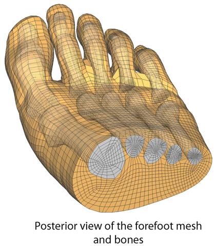
Complexity grows rapidly with dimensions. Consider solving coupled equations on a grid.

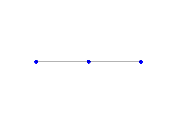
1D Grid

$n$ points. Matrix has ~ $3n$ nonzeros. Tridiagonal (Easy).

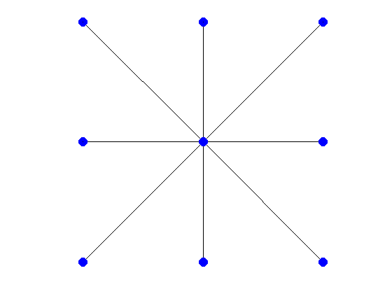
\[ \begin{bmatrix} 2&-1 & & & & \\ & \ddots & & & & \\ & -1 & 2 & -1 & & \\ & & & \ddots & & \\ & & & & -1 & 2 \end{bmatrix} \]

2D Grid

$n^2$ points. ~$9n^2$ nonzeros. $n$-banded (Harder).

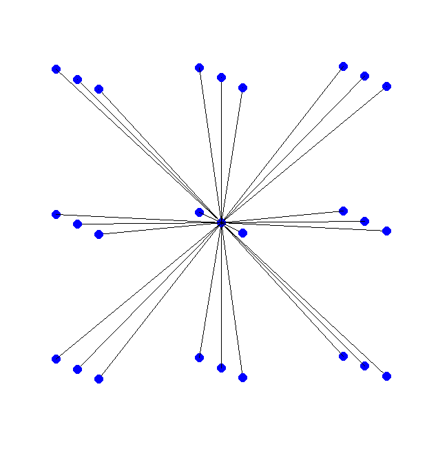
\[ \begin{bmatrix} 8&-1 & & -1 & & \\ & \ddots & & & & \\ -1& -1 & 8 & -1 & -1 & \\ & & & \ddots & & \\ & -1 & & & -1 & 8 \end{bmatrix} \]

3D Grid

$n^3$ points. ~$27n^3$ nonzeros. $n^2$-banded (Yikes!).

Storage Explosion

Dim	Unknowns	Storage
1D	$n$	$3n$
2D	$n^2$	$9n^2$
3D	$n^3$	$27n^3$

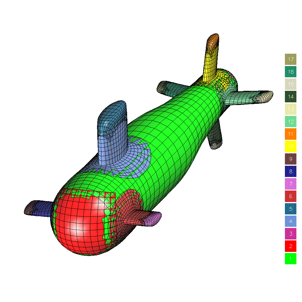
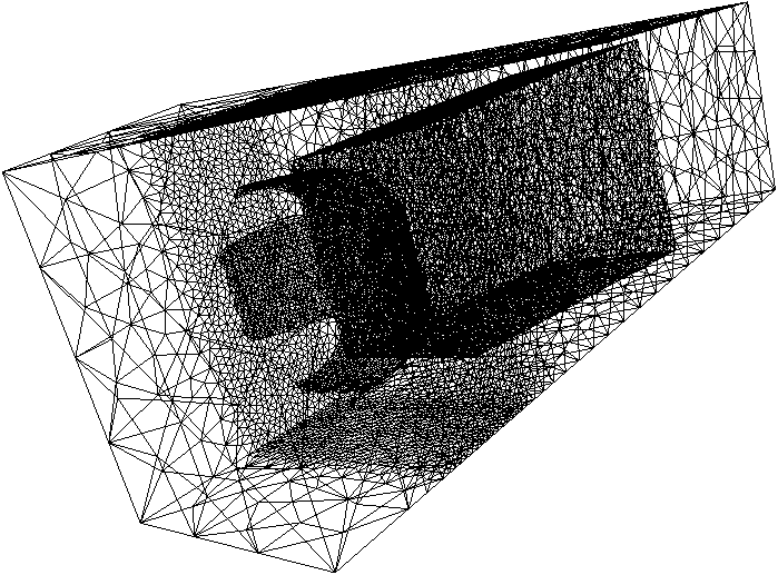
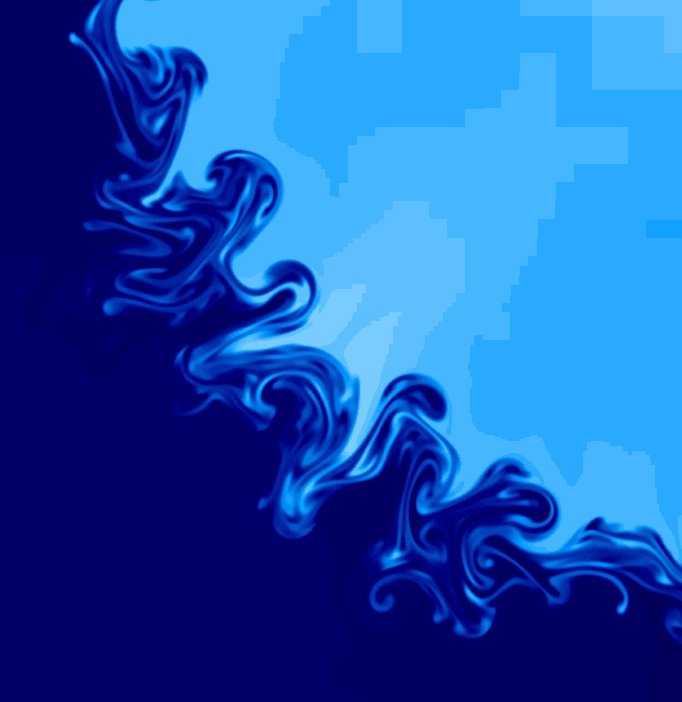
Real World Complexity

4

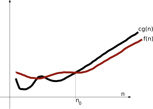
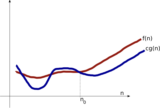
Complexity Analysis (Big-O)

$\mO(g(n))$

Asymptotic Upper Bound

$f(n) \leq c g(n)$

$\Omega(g(n))$

Asymptotic Lower Bound

$c g(n) \leq f(n)$

$\Theta(g(n))$

Asymptotic Tight Bound

$\mO(g(n)) \cap \Omega(g(n))$

5

BLAS & Operations

BLAS (Basic Linear Algebra Subprograms) defines standard interfaces.

Level 1

Vector-Vector

$y \leftarrow \alpha x + y$

Cost: $\mO(n)$

Level 2

Matrix-Vector

$y \leftarrow \alpha A x + \beta y$

Cost: $\mO(n^2)$

Level 3

Matrix-Matrix

$C \leftarrow \alpha A B + \beta C$

Cost: $\mO(n^3)$

Matrix-Vector Multiplication Algorithm

for i = 1...n
    for j = 1...n
        v(i) = a(i,j)*u(j) + v(i)
    end
end

$n^2$ multiplies, $n^2$ additions $\rightarrow \mO(n^2)$

Matrix-Matrix Multiplication Algorithm

for j = 1...n
    for i = 1...n
        for k = 1...n
            C(k,j) = A(k,i)*B(i,j) + C(k,j)
        end
    end
end

$n^3$ multiplies, $n^3$ additions $\rightarrow \mO(n^3)$

6

Gaussian Elimination Schemes

Solving Diagonal Systems

If $A$ is diagonal, the system decouples:

$x_i = b_i / a_{i,i}$

Cost: $\mO(n)$ FLOPS (Cheap!)

% Matlab
A = ... % Diagonal Matrix
x = b ./ diag(A)

Solving Triangular Systems

Lower Triangular ($Ly=b$): Use Forward Substitution.

$x_1 = b_1 / l_{11}$
$x_i = (b_i - \sum l_{ij}x_j) / l_{ii}$

Upper Triangular ($Ux=c$): Use Backward Substitution.

Forward Substitution Algo

x(1) = b(1)/L(1,1)
for i = 2...n
    s = b(i)
    for j = 1...i-1
        s = s - L(i,j)*x(j)
    end
    x(i) = s/L(i,i)
end

Cost Analysis

Total FLOPS $\approx \sum_{j=1}^n 2j = n(n+1) \approx n^2$.

$\mO(n^2)$ FLOPS

7

Interactive Playground

Experiment with matrix operations and timing. You can run MATLAB code via Octave Online or Python code directly in your browser.

MATLAB / Octave (Online)

Copy & Paste into Terminal:

🚀 Open Octave Online

Python (Client-Side)

Output

Loading Python environment...

Linear Algebra Review & Costs