1. Construction of Optimal Control Sequence
Once we have computed the optimal cost-to-go functions \( J^*_k \) using the backward pass, we can construct the optimal control sequence \( \{ u_0^*, \dots, u_{N-1}^* \} \) by moving forward in time.
Forward Pass Algorithm
- Start at \( k=0 \): Find the optimal first control \( u_0^* \) by minimizing: \[ u_0^* \in \arg \min_{u_0 \in U_0(x_0)} \left[ g_0(x_0, u_0) + J_1^*(f_0(x_0, u_0)) \right] \]
- Update State: This takes you to the next state: \[ x_1^* = f_0(x_0, u_0^*) \]
- Iterate Forward: For \( k = 1, 2, \ldots, N-1 \), set: \[ u_k^* \in \arg \min_{u_k \in U_k(x_k^*)} \left[ g_k(x_k^*, u_k) + J_{k+1}^*(f_k(x_k^*, u_k)) \right] \] And update the state: \[ x_{k+1}^* = f_k(x_k^*, u_k^*) \]
2. Illustration of DP with Tail Subproblem
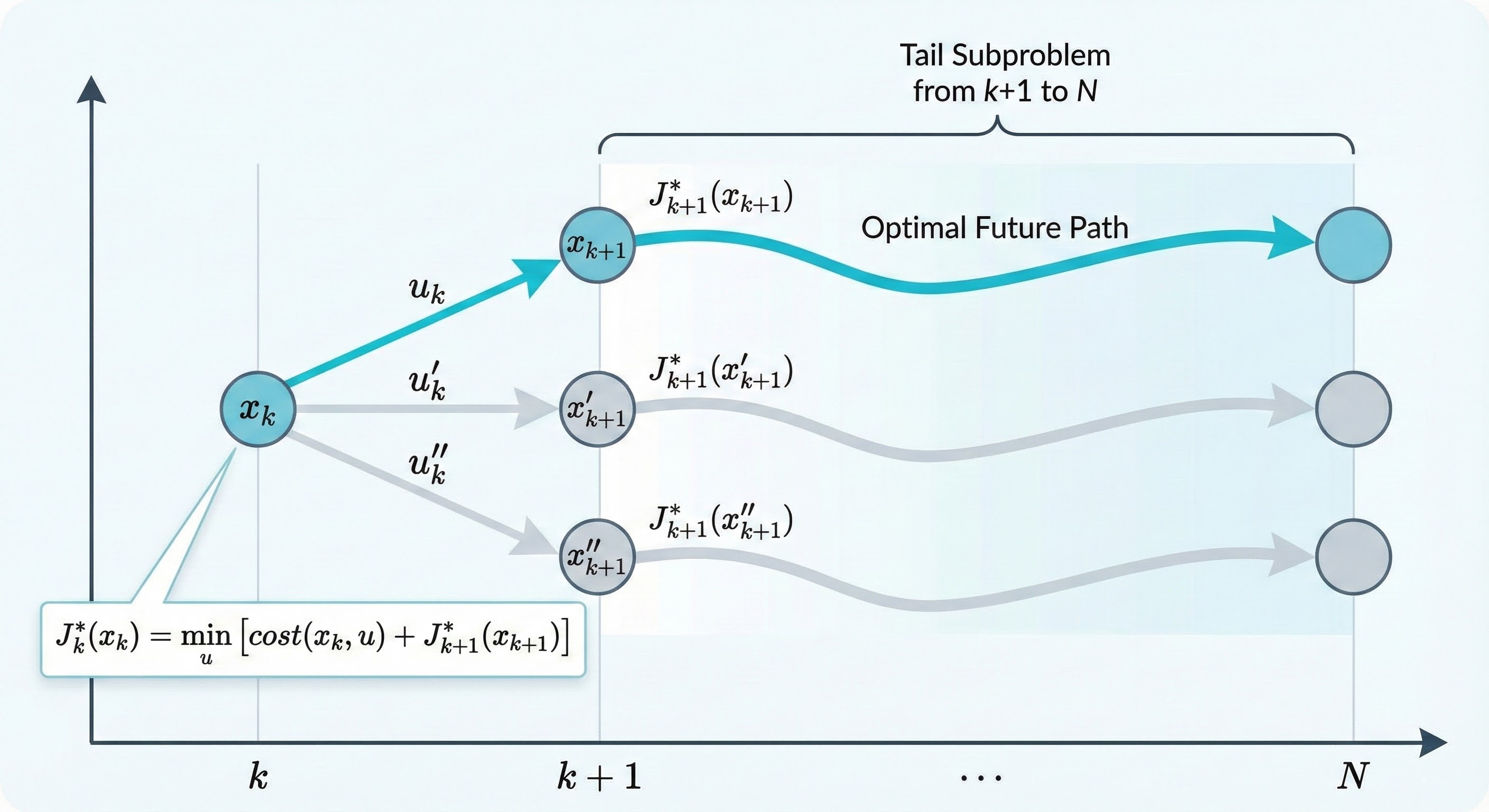
The tail subproblem starts at \( x_k \) at time \( k \) and minimizes over \( \{ u_k, \dots, u_{N-1} \} \).
The Dynamic Programming algorithm can be visualized as solving a sequence of tail subproblems.
- At any state \( x_k \), we look at the "tail" of the problem from time \( k \) to \( N \).
- We assume the future (from \( k+1 \) onwards) is already optimized, represented by \( J^*_{k+1} \).
- We then make the best decision for the current step \( u_k \) to minimize immediate cost plus the optimal future cost.
3. Finite-State Problems: Shortest Path View
Graph Representation
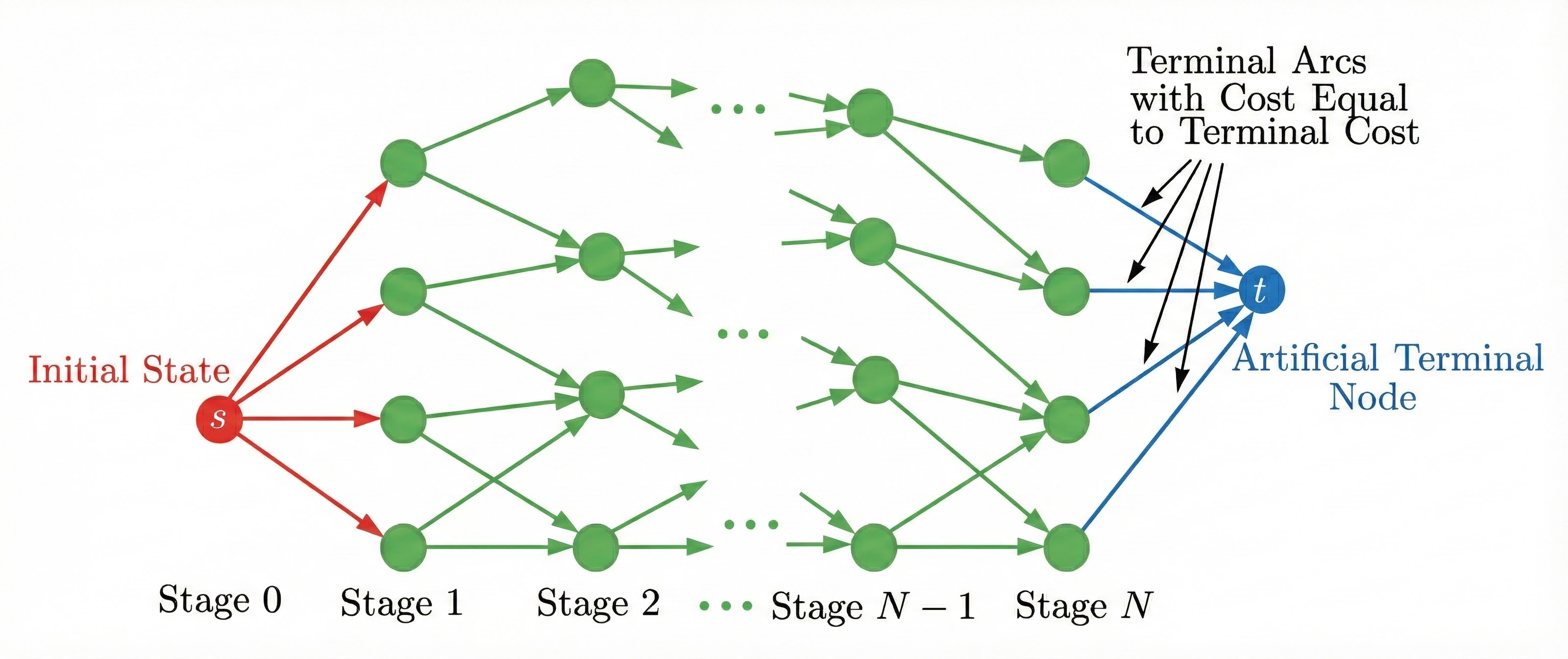
Nodes & Arcs
- Nodes: Correspond to states \( x_k \).
- Arcs: Correspond to state-control pairs \( (x_k, u_k) \).
- An arc \( (x_k, u_k) \) connects node \( x_k \) to node \( x_{k+1} = f(x_k, u_k) \).
Costs & Objective
- Arc Cost: Each arc has a cost \( g(x_k, u_k) \).
- Total Cost: Sum of arc costs from initial node \( s \) to terminal node \( t \).
- Goal: Find the minimum cost path (Shortest Path) from \( s \) to \( t \).
Key Insight:
Any finite-horizon deterministic DP problem with finite states can be viewed as finding the shortest path in a DAG (Directed Acyclic Graph) of states layered by time.
🚧 A Little Detour!
We've established the foundations. Next, we will explore what happens when the horizon goes to infinity!