Lecture 2

Experiments, Matlab & Randomness

Understanding numerical environments, testing methods, and the nature of unpredictability.

Today's Agenda

💻 Get introduced to the basics of Matlab.
🧪 Learn how to test numerical methods, not just run them.
🎲 Investigate randomness and pseudorandom numbers.

The MATLAB Environment

MATrix LABoratory is both a computing environment and a language. Initially an interface to LAPACK (Linear Algebra Package), it is written in C and optimized for matrix computations.

The Good

Fast development times
No compiling (easy debugging)
Accessible syntax
Built-in visualization
Extensive toolboxes

The Bad

Coding mistakes cause slow performance
Loops are computationally intensive
Limited language features (no templates/classes)

The Ugly

Proprietary and expensive
Octave (open source alternative) is not 100% compatible

Interpreter vs. Scripts vs. Functions

Interpreter

Quick access, good for ideas and accessing workspace data. Poor performance and debugging.

Script

Good test bed (all info in workspace), fast and linear. Poor profiling/optimization.

Functions

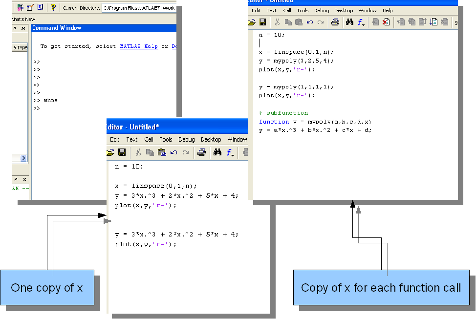
Optimized/cached, reusable. Does not clutter workspace. Pass by value (ouch!).

MATLAB Function Basics

Save in a file named functionname.m.
Can accept 0, $n$, or a variable number of inputs/outputs.
Variables are local by default (scope is limited to the function).
Use global varname to make a variable visible across all functions (use sparingly!).
Use return to exit a function early.

🧠 Knowledge Check +10 XP

Which of the following is a characteristic of MATLAB functions?

Computational Experiments: Taylor Series

How do we evaluate $f(x) = \frac{1}{1-x}$ computationally? We use the Taylor Series Expansion.

Taylor Approximation Error

We truncate the infinite series to a polynomial $p_n(x)$:

\[ f(x) = p_n(x) + E_n(x) \]

The error term $E_n(x)$ is given by:

\[ E_n(x) = \frac{(x-c)^{n+1}}{(n+1)!}f^{(n+1)}(\xi) = \mO(h^{n+1}) \]

Example Calculation

How many terms ($n$) do we need to ensure error $< 2 \times 10^{-8}$ for $x=1/2$?

\[ e_{x=1/2} = \sum_{k=n+1}^{\infty} \left(\frac{1}{2}\right)^k = \frac{(1/2)^{n+1}}{1-1/2} = 2\cdot(1/2)^{n+1} \]

Solving for $n$: $n+1 > \frac{-8}{\log_{10}(1/2)} \approx 26.6 \implies n > 26$.

Measuring Cost: Big-O

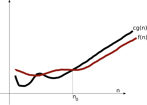
Big-O ($\mO$)

Asymptotic Upper Bound

$\mO(g(n))$: $f(n) \leq c g(n)$ for large $n$.

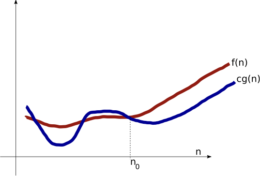
Big-Omega ($\Omega$)

Asymptotic Lower Bound

$\Omega(g(n))$: $c g(n) \leq f(n)$ for large $n$.

Big-Theta ($\Theta$)

Asymptotic Tight Bound

$\Theta(g(n)) = \mO(g(n)) \cap \Omega(g(n))$.

Convergence Rates

Algebraic Convergence

$a_n \sim \mO(1/n^\alpha)$. The sequence converges relatively slowly.

Exponential Convergence

$a_n \sim \mO(e^{-q n^\beta})$. Also known as spectral convergence. Much faster.

Supergeometric: $\beta > 1$
Geometric: $\beta = 1$
Subgeometric: $\beta < 1$

Algorithmic Efficiency

Evaluating polynomials efficiently. Consider $f(x) = 5x^3 + 3x^2 + 10x + 8$.
Standard evaluation: 6 multiplications, 3 additions.

Nested Multiplication (Horner's Method)

Rewrite as: $f(x) = 8 + x(10 + x(3 + x(5)))$

Result: 3 multiplications, 3 additions.

                    p = a_n
                    for i = n-1 to 0 step -1
                    p = a_i + x*p
                    end
                

Randomness

Randomness $\approx$ unpredictability. Computer algorithms are deterministic, so we generate Pseudorandom Numbers.

Case Study: Debian OpenSSL (2008)

A vulnerability in the random number generator meant there were only 32,767 possible keys. All SSL/SSH keys generated over a 2-year period were compromised.

Linear Congruential Generators (LCG)

The standard for many years. Fast, but sensitive to parameters.

\[ x_k = (a x_{k-1} + c) \pmod M \]

Sampling Techniques

Uniform Interval $[a, b)$

To transform a standard uniform sample $x_k \in [0, 1)$ to a generic interval:

\[ r_k = (b-a)x_k + a \]

Non-Uniform (Inversion Method)

If CDF is invertible, we can map uniform samples. E.g., for exponential distribution $f(t) = \lambda e^{-\lambda t}$:

\[ y_k = -\frac{\log(1-x_k)}{\lambda} \]

Properties of Good Generators

Pass statistical tests of randomness
Long period (time before repeating)
Efficiency (speed/memory)
Repeatability (for debugging)

Modern Methods

Mersenne Twister: (Matlab default) Long period.
Method of Marsaglia: Period $\approx 2^{1430}$.
Fibonacci: Uses differences/sums, very good statistical properties.

Quasi-Random Sequences

Sometimes "true" randomness clumps together. Quasi-random sequences are designed to avoid clumping for better coverage of the sample space.

🧠 Final Challenge +20 XP

Why is Repeatability considered a desirable property for a Random Number Generator in scientific computing?