About Functions
We will mostly deal with functions with domain and co-domain subsets of \( \mathbb{R} \).
📐 Types of Functions
1. Real-valued, Single Variable
\[ f: \mathbb{R} \rightarrow \mathbb{R} \]Example: \( f(x) = x^2 \)
2. Real-valued, Multi-variable
\[ f: \mathbb{R}^n \rightarrow \mathbb{R} \]Example: \( f(x,y) = x^2 + y^2 \)
3. Vector-valued, Multi-variable
\[ f: \mathbb{R}^n \rightarrow \mathbb{R}^m \]Example: \( f(x,y) = (x^2, \exp(x+y), \sin(x)) \)
💡 More Examples
- \( f(x) = x, \quad x \in \mathbb{R} \)
- \( f(x) = \max(x), \quad x \in \mathbb{R}^n \)
- \( f(x,y) = x^2 + y^2 \)
- \( f(A) = \text{det}(A), \quad A \in \mathbb{R}^{n \times n} \)
- \( f(x,y) = (x^2, \exp(x+y), \sin(x)) \)
What is a Gradient?
📊 Gradient Definition
For a real-valued function:
\[ f: \mathbb{R}^n \rightarrow \mathbb{R} \]The gradient is the vector of partial derivatives:
\[ \nabla f = \begin{pmatrix} \dfrac{\partial f}{\partial x_1} \\ \dfrac{\partial f}{\partial x_2} \\ \dfrac{\partial f}{\partial x_3} \\ \vdots \\ \dfrac{\partial f}{\partial x_n} \end{pmatrix} \in \mathbb{R}^n \]✍️ Exercise: Compute Gradients
Try computing the gradients for these functions:
1. \( f(x,y) = x^2 + y^2 \)
2. \( f(x,y) = x - y \)
Gradient of Vector-Valued Functions: The Jacobian
What happens when our function outputs a vector instead of a scalar?
🔷 Jacobian Matrix
For a vector-valued function:
\[ f: \mathbb{R}^n \rightarrow \mathbb{R}^m \]We can view this as:
\[ f\begin{pmatrix} x_1 \\ \vdots \\ x_n \end{pmatrix} = \begin{pmatrix} f_1(x) \\ \vdots \\ f_m(x) \end{pmatrix} \]The Jacobian matrix \( J \in \mathbb{R}^{m \times n} \) is:
\[ J = \begin{pmatrix} \dfrac{\partial f_1}{\partial x_1} & \dots & \dfrac{\partial f_1}{\partial x_n} \\ \vdots & \ddots & \vdots \\ \dfrac{\partial f_m}{\partial x_1} & \dots & \dfrac{\partial f_m}{\partial x_n} \end{pmatrix} \]Why Gradients?
🔴 Question
Why are we interested in gradients?
📘 Fact from Calculus
Gradients point in the direction of greatest increase of the function!
✅ Answer
Hence, \( -\nabla f(x) \) gives the direction of descent. This helps us find local minima!
Gradient vectors perpendicular to level curves
🎯 Three Key Questions
- What is a level curve?
- Where does \( \nabla \) point to?
- How does gradient help in going to minima?
We'll answer each of these in detail!
1. Level Curves
📍 Level Curve Definition
The level curve of a scalar-valued function:
\[ f: \mathbb{R}^n \rightarrow \mathbb{R} \]is defined as the set:
\[ f_t = \{(x,y) \mid f(x,y) = t, \quad t \in \mathbb{R}\} \]These are the curves where the function has constant value \( t \).
✏️ Quiz: Draw Level Curves
Can you visualize the level curves for these functions?
1. \( f(x,y) = x^2 + y^2 \) for \( t = 0, 1, 2 \)
Answer: Concentric circles!
- \( t = 0 \): A point at the origin
- \( t = 1 \): Circle with radius 1
- \( t = 2 \): Circle with radius \( \sqrt{2} \)
2. \( f(x,y) = x^2 - y^2 \) for \( t = 0, 1, 2 \)
Answer: Hyperbolas!
- \( t = 0 \): Lines \( y = \pm x \) (degenerate hyperbola)
- \( t = 1 \): Hyperbola opening left-right
- \( t = 2 \): Wider hyperbola
Level curves are convenient for showing directions towards minima/maxima
2. Gradient is Perpendicular to Level Curves
🎓 Theorem
The gradient vector \( \nabla f \) points in the direction perpendicular to the tangent drawn on the level curve.
🔍 Proof (2D Case)
Proof for 2D functions: \( w = f(x,y) \). Let \( f(x,y) = c \) be a level curve.
Step 1: Apply Implicit Function Theorem
By the implicit function theorem, we can write:
\[ y = y(x) \]Step 2: Level curves become
\[ f(x, y(x)) = c \]Step 3: Apply Chain Rule
Differentiating both sides with respect to \( x \):
\[ \dfrac{\partial f}{\partial x} + \dfrac{\partial f}{\partial y} \dfrac{dy}{dx} = 0 \]Therefore:
\[ \dfrac{dy}{dx} = -\dfrac{\partial f / \partial x}{\partial f / \partial y} \]Step 4: Find Tangent Vector
The tangent vector to the level curve is:
\[ t = \begin{pmatrix} 1 \\ dy/dx \end{pmatrix} = \begin{pmatrix} 1 \\ -\frac{\partial f / \partial x}{\partial f / \partial y} \end{pmatrix} \]Or equivalently (multiplying by \( \partial f / \partial y \)):
\[ t \propto \begin{pmatrix} -\partial f / \partial y \\ \partial f / \partial x \end{pmatrix} \]Step 5: Compare with Gradient
The gradient is:
\[ \nabla f = \begin{pmatrix} \partial f / \partial x \\ \partial f / \partial y \end{pmatrix} \]Step 6: Check Perpendicularity
Compute the dot product:
\[ t \cdot \nabla f = (-\partial f / \partial y)(\partial f / \partial x) + (\partial f / \partial x)(\partial f / \partial y) = 0 \]Since the dot product is zero, \( \nabla f \perp t \). ∎
3. Gradient Descent Algorithm for Minima
🔴 Question: How does gradient help in going to minima?
📘 Answer: Just follow the descent direction, i.e., negative of gradient!
🔧 Gradient Descent (GD) Algorithm
Step 1: Start from initial guess
\[ x^0 \in \mathbb{R}^n \]Step 2: Iterate - move in descent direction
\[ x^{i+1} \leftarrow x^i - t \nabla f(x^i), \quad i = 0, 1, 2, \dots \]where \( t > 0 \) is the step size (or learning rate) that tells how far to move
Step 3: Stopping Criteria
Stop when:
- Gradient is "flat": \( \|\nabla f(x^i)\| \approx 0 \) (at least machine precision)
- Or, position doesn't change: \( \|x^i - x^{i-1}\| \) is "small enough"
Step 4: Return minimizer
Return \( x^i \) as the local minimum
📈 Gradient Ascent Algorithm for Maxima
To find maxima instead, just change the sign!
Update Rule:
\[ x^{i+1} \leftarrow x^i + t \nabla f(x^i), \quad i = 0, 1, 2, \dots \]Note the + sign: we move in the direction of the gradient!
🎯 Quiz 1: Gradient Descent Understanding
What is the key difference between gradient descent and gradient ascent?
Gradient Descent History: Augustin-Louis Cauchy
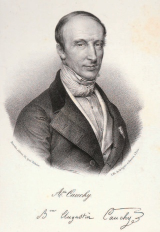
Baron Augustin-Louis Cauchy (1789-1857)
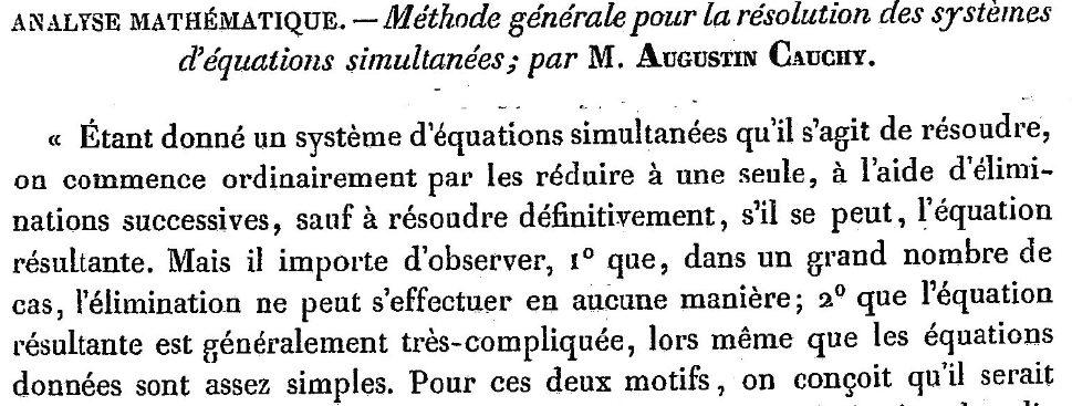
📜 Original Paper (1847)
Title: Methode generale pour la resolution des systemes d'equations simultanees
Translation: "General method for resolution of systems of simultaneous equations"
Published in: C. R. Acad. Sci. Paris, 25:536–538, 1847
📖 Review of Cauchy's Original Paper
🇫🇷 Translation (Introduction)
"Given a system of simultaneous equations that we want to solve, we usually start with successive elimination of variables. However, it is important to observe that:
- In many cases, eliminations cannot be done in any manner.
- The resulting equations during eliminations are, in general, very complicated, even though the given equations are essentially simple..."
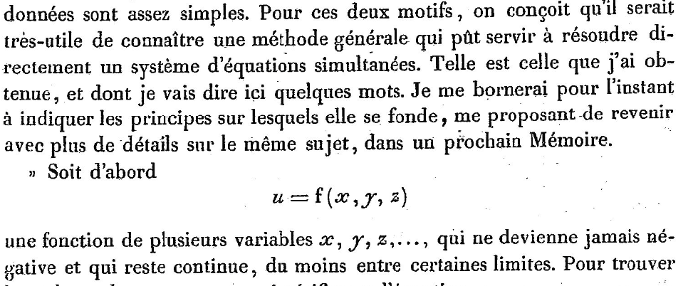
🇫🇷 Translation (The Method)
"Given these two points, we believe that it will be very useful to know one general method that can resolve a simultaneous system of equations. This is what I have got, and I am going to say a few words."
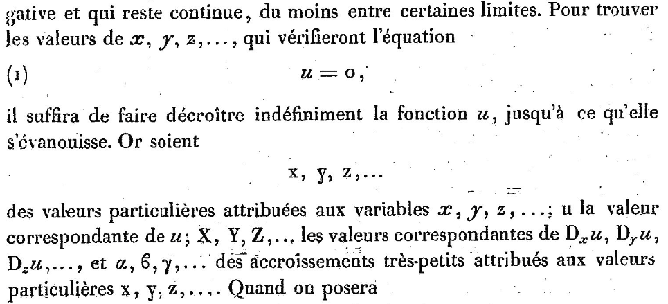
"First of all, let \( u = f(x,y,z,\dots) \) be a function of several variables \( x, y, z, \dots \) that is never negative and is continuous at least within certain limits..."
🔬 Cauchy's Key Insight
"To find the values \( x, y, z, \dots \) that will verify the equation \( u = 0 \), it will suffice to do an indefinite decrease of the function \( u \), until it vanishes."
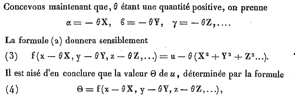
Cauchy's Update Rule:
Let \( \alpha, \beta, \gamma \) be small values. When we set:
\[ \alpha = -\theta X, \quad \beta = -\theta Y, \quad \gamma = -\theta Z \]where \( X, Y, Z \) are \( D_x u, D_y u, D_z u \), we get:
\[ f(x - \theta X, y - \theta Y, z - \theta Z, \dots) = u - \theta(X^2 + Y^2 + Z^2 + \dots) \]Since we subtract a positive quantity from \( u \), the function is decreasing! This is gradient descent!
🔍 Spot the Mistake!
Find the error in this "proof" that gradient descent always finds the global minimum:
1. Gradient descent follows the direction -∇f(x).
2. This direction points toward lower values of f.
3. Therefore, gradient descent will always reach the global minimum of f.
4. The algorithm stops when ∇f(x) ≈ 0.
When is Gradient Descent Guaranteed to Work?
🎓 Key Question
For which functions is GD guaranteed to find extrema (maxima or minima)?
Conditions for Convergence:
- Convex Functions: For minimization, if \( f \) is convex, GD finds the global minimum
- Concave Functions: For maximization, if \( f \) is concave, gradient ascent finds the global maximum
- Smooth Functions: \( f \) should be differentiable with Lipschitz continuous gradient
- Appropriate Step Size: \( t \) must be small enough for convergence
⚠️ Warning: Non-Convex Functions
For non-convex functions (like most neural network loss functions!), gradient descent may:
- Get stuck in local minima
- Get stuck at saddle points
- Depend heavily on initialization
This is why modern optimization uses variants like SGD, Adam, RMSProp, etc.!
🎯 Quiz 2: Advanced Questions
1. Why is the gradient perpendicular to level curves?
2. What happens if the step size t is too large in gradient descent?
Summary
🔢 Functions & Gradients
Gradients are vectors of partial derivatives that point in the direction of greatest increase
🗺️ Level Curves
Curves where function has constant value; gradients are perpendicular to them
⬇️ Gradient Descent
Iterative algorithm: x^(i+1) = x^i - t∇f(x^i) finds minima by following descent direction
👨🔬 History
Cauchy invented gradient descent in 1847 for solving systems of equations
✅ When It Works
Guaranteed for convex/concave functions; local minima for non-convex
🎛️ Jacobian
Matrix of partial derivatives for vector-valued functions (m × n)
🎓 The Big Picture
Optimization is at the heart of machine learning! Gradient descent and its variants (SGD, Adam, etc.) power the training of neural networks, making modern AI possible. Understanding the mathematics—from gradients and level curves to Cauchy's original insight—gives you deep intuition for how these algorithms work and when they succeed!