1. Introduction to Time Delays
Definition
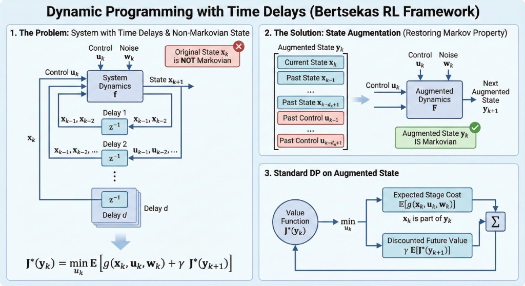
In many applications, the next state \(x_{k+1}\) is influenced not just by \(x_k\) and \(u_k\), but also by previous states \(x_{k-1}, \dots\) and controls \(u_{k-1}, \dots\).
Consider a system with at most one stage delay:
\[ x_{k+1} = f_k(x_k, x_{k-1}, u_k, u_{k-1}) \]System with Delay
2. State Augmentation
We can transform this into a standard system by introducing new state variables:
\[ y_k = x_{k-1}, \quad z_k = u_{k-1} \]Augmented State Vector
Define the new state \(\tilde{x}_k = (x_k, y_k, z_k)\). The system becomes:
\[ \tilde{x}_{k+1} = \tilde{f}_k(\tilde{x}_k, u_k, w_k) \]Augmented State Visualization
3. DP Algorithm with Delays
By expressing the cost in terms of \(\tilde{x}_k\), we get a problem without delays. The policy \(\mu_k\) now depends on \((x_k, x_{k-1}, u_{k-1})\).
Reformulated Bellman Equation
\[ J^*_k(x_k, x_{k-1}, u_{k-1}) = \min_{u_k} E_{w_k} \left[ g_k + J^*_{k+1}(f_k(\dots), x_k, u_k) \right] \]4. Non-additive Cost Structures
In extreme cases, cost might depend on the entire history:
\[ E\{g_N(x_N, \dots, x_0, u_{N-1}, \dots, u_0)\} \]We augment the state to include the entire history:
\[ \tilde{x}_k = (x_k, \dots, x_0, u_{k-1}, \dots, u_0) \]5. Summary Infographic
6. Test Your Knowledge
1. To handle a 1-step time delay in state \(x_{k-1}\), we augment the state with:
2. If the control \(u_{k-1}\) affects \(x_{k+1}\), the policy \(\mu_k\) must depend on:
3. State augmentation transforms a delayed system into:
4. For non-additive costs depending on full history, the state dimension:
5. Can we handle delays in disturbances \(w_{k-1}\)?
🔍 Spot the Mistake!
Scenario 1:
"We can ignore past controls \(u_{k-1}\) if only \(x_{k-1}\) affects the dynamics."
Scenario 2:
"Augmenting the state reduces the computational complexity."
Scenario 3:
"The cost function must always be additive for DP to work."