1. Introduction
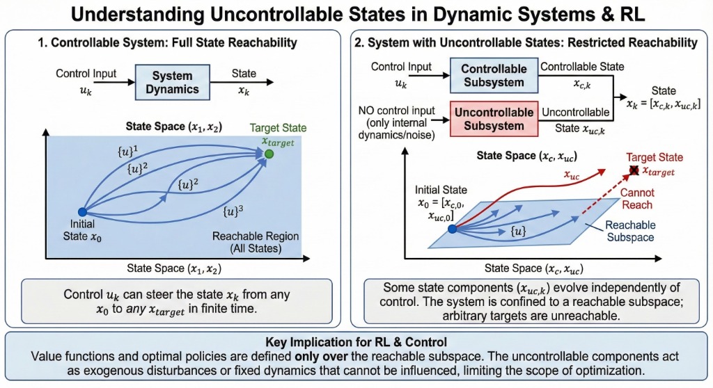
In many problems, the state consists of two types of components:
- Controllable \(x_k\): Affected by control \(u_k\).
- Uncontrollable \(y_k\): Unaffected by control \(u_k\) (except via \(x_k\)).
System Dynamics
\[ x_{k+1} = f_k(x_k, y_k, u_k, w_k) \]\(y_k\) evolves according to a given conditional distribution \(P_k(y_k | x_k)\).
State Components
2. Averaging Out Uncontrollable Components
Key Insight: We can structure DP to operate primarily on the controllable component \(x_k\), "averaging out" \(y_k\).
Average Cost-to-Go
Define \(\hat{J}_k(x_k)\) as the expected optimal cost given only \(x_k\):
\[ \hat{J}_k(x_k) = E_{y_k} \{J^*_k(x_k, y_k) | x_k\} \]3. Simplified DP Algorithm
The DP algorithm for \(\hat{J}_k(x_k)\) operates on a reduced state space (only \(x_k\)).
Simplified Bellman Equation
\[ \hat{J}_k(x_k) = E_{y_k} \left\{ \min_{u_k} E_{w_k} \left\{ g_k(x_k, y_k, u_k, w_k) + \hat{J}_{k+1} (f_k(\dots)) \mid x_k, y_k, u_k \right\} \mid x_k \right\} \]This is advantageous because approximating \(\hat{J}_k(x_k)\) is typically easier than approximating the full \(J^*_k(x_k, y_k)\).
4. Application to Forecasts
Recall the Forecast example from Lecture 07. The forecast \(y_k\) is an uncontrolled state component.
If \(y_k\) takes values \(i = 1, \dots, m\) with probability \(p_i\), the algorithm simplifies to:
\[ \hat{J}_k(x_k) = \sum_{i=1}^{m} p_i \min_{u_k} E_{w_k} \left\{ g_k + \hat{J}_{k+1}(f_k(\dots)) \mid y_k = i \right\} \]This runs over the space of \(x_k\) only, not the combined \((x_k, y_k)\)!
5. Test Your Knowledge
1. An uncontrollable state component \(y_k\) is:
2. Is \(y_k\) the same as a disturbance \(w_k\)?
3. The simplified DP algorithm computes:
4. The main advantage of this approach is:
5. In the forecast example, the simplified state is:
🔍 Spot the Mistake!
Scenario 1:
"Since \(y_k\) is uncontrollable, we can just ignore it completely."
Scenario 2:
"The optimal control \(u_k\) depends only on \(x_k\) in the simplified problem."
Scenario 3:
"This simplification works even if \(y_k\) is affected by \(u_{k-1}\)."