1. Constructing \( \tilde{J}_k \)
A major challenge in value space approximation is constructing suitable approximate cost-to-go functions \( \tilde{J}_k \). This can be done in various ways:
Off-line Training
Constructing \( \tilde{J}_k \) using sophisticated training methods (e.g., Neural Networks) before the decision process begins.
On-line Rollout
Obtaining \( \tilde{J}_k(x_k) \) when needed by running a heuristic control scheme, called a base heuristic or base policy.
2. The Rollout Algorithm
High-Level Plan
Given a state \( x_k \) at time \( k \), the algorithm considers all tail subproblems starting at every possible next state \( x_{k+1} \), and solves them suboptimally by using a base heuristic.
Detailed Steps
- Generate Next States: At \( x_k \), consider all possible controls \( u_k \in U_k(x_k) \) and generate the corresponding next states \( x_{k+1} \).
- Run Base Heuristic: From each \( x_{k+1} \), simulate the system forward using the base heuristic to generate a sequence of states and controls up to the terminal stage \( N \): \[ x_{t+1} = f_t(x_t, u_t), \quad t = k, \dots, N - 1 \]
- Calculate Heuristic Cost: Accumulate the costs incurred during this simulation to get \( H_{k+1}(x_{k+1}) \): \[ H_{k+1}(x_{k+1}) = g_{k+1}(x_{k+1}, u_{k+1}) + \dots + g_{N-1}(x_{N-1}, u_{N-1}) + g_N(x_N) \]
- Minimization: Select the control \( u_k \) that minimizes the immediate cost plus the heuristic cost: \[ \tilde{u}_k = \arg\min_{u_k \in U_k(x_k)} \left[ g_k(x_k, u_k) + H_{k+1}(f_k(x_k, u_k)) \right] \]
3. Q-Factor Formulation
We can express the rollout algorithm more succinctly using approximate Q-factors.
The rollout algorithm applies the control \( \mu_k(x_k) \) given by:
\[ \mu_k(x_k) \in \arg \min_{u_k \in U_k(x_k)} \tilde{Q}_k(x_k, u_k) \]where the approximate Q-factor is defined as:
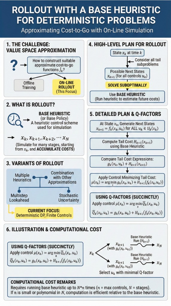
\[ \tilde{Q}_k(x_k, u_k) = g_k(x_k, u_k) + H_{k+1}(f_k(x_k, u_k)) \]4. Visual Illustration
Fig: The rollout process. For each possible control, we simulate the future using the base heuristic to estimate the "tail cost", then pick the best option.
5. Computational Complexity
How expensive is it?
- The algorithm runs the base heuristic at most \( N \times n \) times, where \( n \) is the max number of controls at each state.
- If \( n \) is small relative to \( N \), the cost is just a small multiple of \( N \) times the base heuristic cost.
- If \( n \) is polynomial in \( N \), the total ratio is also polynomial in \( N \).
Key Takeaway: Rollout is generally computationally feasible if the base heuristic is fast.